I had low tire pressure yesterday due to the polar vortex, so I added additional air to my tires to about 34PSI at 22F, today it is much warmer at nearly 50F and the PSI went up more than I expected. Also the PSI doesn’t seem to change as much from Spring to Summer, when the weather can swing up more than 20 degrees from night to day. I decided to write some python to try to figure this whole thing out using the Ideal Gas Law. Also no attempt was made to account for the weight of the car, and how that adds pressure to tire.

The equation terms mean the following with their SI units in parenthesis.

• $P$ is the pressure. (pascals)
• $V$ is the volume. (meters³)
• $n$ is the number of moles of gas. (unit less)
• $R$ is the ideal gas constant
• $T$ is the temperature in kelvins.

We have a couple of things we need to solve. The first part is the number of moles of gas in my tires. From there we can figure out how changing the temperature affects the pressure and attempt to attribute how much the expansion of my tires due to heat affects the pressure.

Unit Conversions

The most important thing about physics and math in this situation is making sure your units line up correctly and are in metric. I have to do a couple of conversions to get everything to line up properly.

The first couple are conversions from US imperial to metric in size. The next is using pascals, does that helps with making sure the numbers line up in a logical manner and prevents boneheaded mistakes.

import math

R = 8.31446261815324 # Ideal Gas Constant m3⋅Pa⋅K−1⋅mol−1

def inches2meters(inches):
    return inches * 0.0254

def psi2Pascal(psi):
    return psi * 6894.7572932

def pascal2Psi(pascals):
    return pascals / 6894.7572932

We should test our unit conversion function to make sure it lines up as we expect. If we convert back and forth, we should receive roughly the same number, and we do.

psi = 36.0
pascals = psi2Pascal(psi)

psi, pascal2Psi(pascals)

(36.0, 36.0)

We also need to convert from the imperial units of temperature to Kelvins.

def fDegrees2Kelvins(f):
    return f * (9.0 / 5.0) + 273.15

Next we have to calculate the volume of the tire. I plugged in some numbers that sound right for my car.

def volume_of_tire(major, minor, width):
    # Area of circle is PI*r^2
    # Volume of Cylinder is PI*r^2*height
    outer = math.pi * major * major
    inner = math.pi * minor * minor
    return (outer - minor) * width

tire_volume_m3 = volume_of_tire(inches2meters(24), inches2meters(20), inches2meters(5))
tire_volume_m3

0.0837506620437606

Now that the tire size is in meters cubed, we can calculate the moles from the known quantities I got today from the tire pressure measurement system. Today it was 44F, and my tire had about 39PSI in it.

def moles(p, v, tk):
    return (p * v) / (R * tk)

moles_of_gas = moles(psi2Pascal(psi), tire_volume, fDegrees2Kelvins(44))
moles_of_gas

7.095798455289843

The next step is to characterize how the temperature yesterday affected my tire pressure. It was about 14F.

def pressure(moles, temp, volume):
    return (moles * R * temp) / volume

pascals = pressure(moles_of_gas, fDegrees2Kelvins(14), tire_volume)
pascal2Psi(pascals)

30.482758620689655

So, just a small drop in temperature of 20 degrees is enough to decrease the PSI by 6. This seems like an awful lot, but we did not account for volumetric shift due to the cold.

Volume Calculations

The next step is to determine the expansion and contraction of the tire rubber with respect to temperature. I’m going to compute all volume changes with respect to the tire measurements in linear units rather than volume, because that feels right and its easier to find unit formulas. I found constants ($\alpha$) for thermal expansion at this handy site.

The units for this are $meters * 10^{-6} / (meters * degreeC)$. This is because the change is typically so small. We don’t have to convert to Celsius because kelvins are Celsius with a different zero point.

STD_TEMP = fDegrees2Kelvins(44)
RUBBER_ALPHA = 80 * 1e-6

def d_length_at_tk(l0, new_temp):
    return l0 * RUBBER_ALPHA * (new_temp - STD_TEMP)

d_length_at_tk(inches2meters(24), fDegrees2Kelvins(100))

0.004915814399999999

As we can see the change in length is very small, but it might have some impact in the overall change in pressure, so let’s calculate it out. I’m going to define a class to help with the volume calculations.

from dataclasses import dataclass

@dataclass
class Tire:
    major : float
    minor : float
    width : float
    
    def normal_volume(self):
        return volume_of_tire(self.major, self.minor, self.width)
    
    def volume_at_temp(self, temp):
        major_axis = self.major + d_length_at_tk(self.major, temp)
        minor_axis = self.minor + d_length_at_tk(self.minor, temp)
        width_axis = self.width + d_length_at_tk(self.width, temp)
        return volume_of_tire(major_axis, minor_axis, width_axis)
    
my_tire = Tire(inches2meters(24), inches2meters(20), inches2meters(5))

# Little test to see if answers remain the same
my_tire.normal_volume() == myTire.volume_at_temp(STD_TEMP)

True

my_tire.normal_volume(), my_tire.volume_at_temp(fDegrees2Kelvins(100))

(0.0837506620437606, 0.08632182197652641)

Volume vs Temperature Plot

import matplotlib.pyplot as plt

xticks = [x for x in range(-20, 110, 1)]
temps = [fDegrees2Kelvins(x) for x in xticks]
volumes = [my_tire.volume_at_temp(t) for t in temps]

fig, ax = plt.subplots()

ax.set_xlabel("Temperature (degrees F)")
ax.set_ylabel("Volume (meters^3)")

plt.plot(xticks, volumes)
plt.show()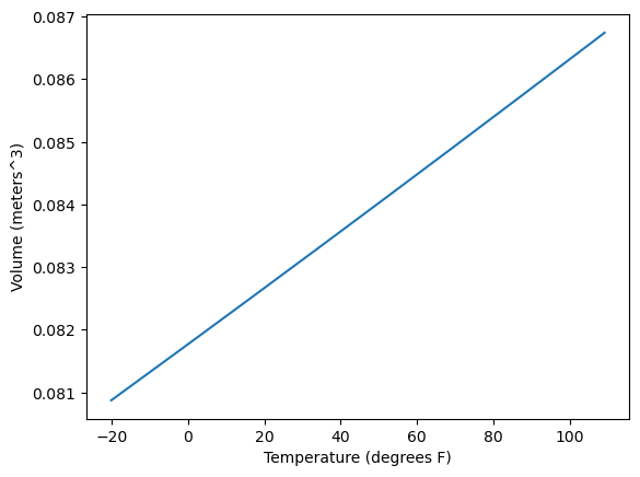

Building the new model

The next step is to define a function that takes into account the change in volume due to temperature.

def tire_pressure(moles, temp, tire):
    volume = tire.volume_at_temp(temp)
    return (moles * R * temp) / volume
    

It’s time for some plots, and to see how much the change in volume affects everything. The temperature range I’m interested in from -20 Fahrenheit to a 110 degrees.

I’m also interested in what my car actually reported, but I’m going based off of my memory since I didn’t write them down. This whole post is about me trying to build a model, when the car’s monitoring felt way off.

import matplotlib.pyplot as plt



pressures_with_volume = [pascal2Psi(tire_pressure(moles_of_gas, t, my_tire)) for t in temps]


fig, ax = plt.subplots()

ax.set_xlabel("Temperature (degrees F)")
ax.set_ylabel("Pressure (PSI)")

plt.plot(xticks, pressures_with_volume, label='volume_model')

pressures = [pascal2Psi(pressure(moles_of_gas, t, tire_volume_m3)) for t in temps]

plt.plot(xticks, pressures, label='naive')

tpsm_temps = [14, 20, 44]
tpsm_psi   = [30, 31, 39]

plt.plot(tpsm_temps, tpsm_psi, label='actual tpsm measurements', marker='o', linestyle='dashed')

plt.legend()
plt.show()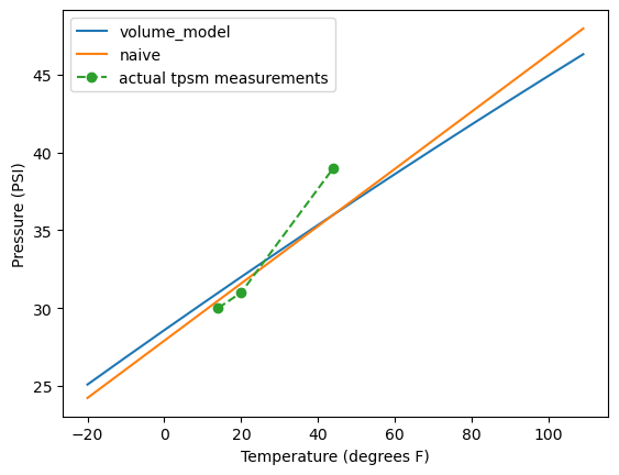

Interpretation

As can be seen in the plot above, either my model isn’t very good or the tire pressure monitoring system (TPMS) isn’t good in my car. I’m leaning towards the TPMS in my car being relatively inaccurate, as I don’t drive a very high end car. It seemed to be all over the place today as it warmed up today from the polar vortex.

Assumptions

There’s a couple key assumptions that have been made with this analysis and spots where error can occur. I’m honestly not sure how to control for these issues, but I don’t think they matter for my overall analysis.

1. I was going from memory when I grabbed these reading from the dashboard and placed them in the plot.
2. The tire might have leaked some amount of gas as it warmed up.
3. I did not test over a wide enough temperature range, only during the day as it warmed up.
4. My volume calculations might be incorrect and overly simplified. A real tire is kind of curved on the sidewalls, and do not have right angles with the surface.
5. I should have checked against a real tire pressure meter from the auto parts store for a complete picture. Although this has confounding factors by removing some number of gas molecules for each measurement.

Thank you for your attention and careful reading. I certainly found it interesting to put into practice the things I learned in high school, and apply it to the real world. Many times we don’t put enough work into synthesizing our existing knowledge into new fields and real problems. It’s important to be able to say when the math doesn’t feel right to you, and validate it against your assumptions and a known physical model.

You can find this notebook on my GitHub.